Note

This tutorial is generated from a Jupyter notebook that can be downloaded and run interactively.

📓 Download notebook

Working with NumPy

All data structures in CloudViewer are natively compatible with a NumPy buffer. The following tutorial generates a variant of sync function using NumPy and visualizes the function using CloudViewer.

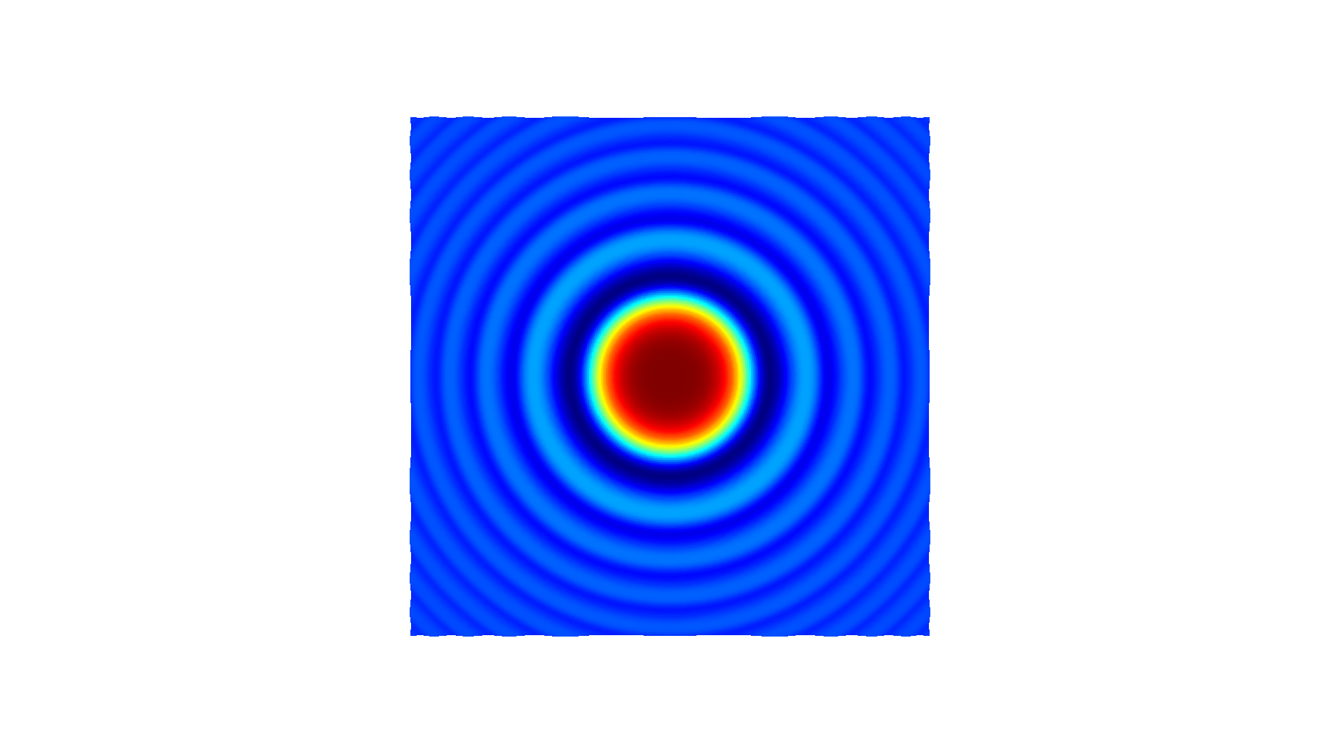
First, we generate a \(n \times 3\) matrix xyz. Each column has \(x\), \(y\), and \(z\) values of the function \(z = \frac{sin(x^2 + y^2)}{x^2 + y^2}\). \(z_\text{norm}\) is the normalized map of \(z\) for the [0,1] range.

# Generate some neat n times 3 matrix using a variant of sync function
x = np.linspace(-3, 3, 401)
mesh_x, mesh_y = np.meshgrid(x, x)
z = np.sinc((np.power(mesh_x, 2) + np.power(mesh_y, 2)))
z_norm = (z - z.min()) / (z.max() - z.min())
xyz = np.zeros((np.size(mesh_x), 3))
xyz[:, 0] = np.reshape(mesh_x, -1)
xyz[:, 1] = np.reshape(mesh_y, -1)
xyz[:, 2] = np.reshape(z_norm, -1)
print('xyz')
print(xyz)

xyz
[[-3.         -3.          0.17846472]
 [-2.985      -3.          0.17440115]
 [-2.97       -3.          0.17063709]
 ...
 [ 2.97        3.          0.17063709]
 [ 2.985       3.          0.17440115]
 [ 3.          3.          0.17846472]]

From NumPy to cloudViewer.ccPointCloud

CloudViewer provides conversion from a NumPy matrix to a vector of 3D vectors. By using Vector3dVector, a NumPy matrix can be directly assigned to cloudViewer.ccPointCloud.points.

In this manner, any similar data structure such as cloudViewer.ccPointCloud.colors or cloudViewer.ccPointCloud.normals can be assigned or modified using NumPy. The code below also saves the point cloud as a ply file for the next step.

# Pass xyz to CloudViewer.cv3d.geometry.ccPointCloud and visualize
pcd = cv3d.geometry.ccPointCloud()
pcd.set_points(cv3d.utility.Vector3dVector(xyz))
cv3d.io.write_point_cloud("sync.ply", pcd)

True

From cloudViewer.ccPointCloud to NumPy

As shown in this example, pcd_load.points of type Vector3dVector is converted into a NumPy array using np.asarray.

# Load saved point cloud and visualize it
pcd_load = cv3d.io.read_point_cloud("sync.ply")

# Convert CloudViewer.cv3d.geometry.ccPointCloud to numpy array
xyz_load = np.asarray(pcd_load.get_points())
print('xyz_load')
print(xyz_load)
cv3d.visualization.draw_geometries([pcd_load])
os.remove("sync.ply")

xyz_load
[[-3.         -3.          0.17846473]
 [-2.9849999  -3.          0.17440115]
 [-2.97000003 -3.          0.17063709]
 ...
 [ 2.97000003  3.          0.17063709]
 [ 2.9849999   3.          0.17440115]
 [ 3.          3.          0.17846473]]
[CloudViewer WARNING] GLFW Error: X11: The DISPLAY environment variable is missing
[CloudViewer WARNING] GLFW initialized for headless rendering.