Note
This tutorial is generated from a Jupyter notebook that can be downloaded and run interactively.
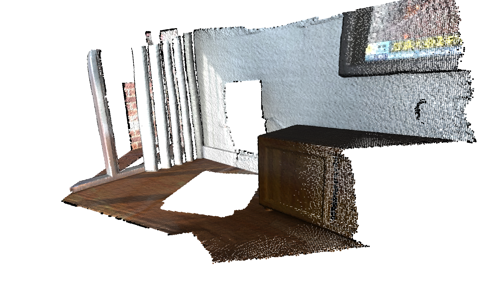
Point cloud#
This tutorial demonstrates basic usage of a point cloud.
Visualize point cloud#
The first part of the tutorial reads a point cloud and visualizes it.
[2]:
print("Load a ply point cloud, print it, and render it")
ply_point_cloud = cv3d.data.PLYPointCloud()
pcd = cv3d.io.read_point_cloud(ply_point_cloud.path)
print(pcd)
print(np.asarray(pcd.get_points()))
cv3d.visualization.draw_geometries([pcd],
                                   zoom=0.3412,
                                   front=[0.4257, -0.2125, -0.8795],
                                   lookat=[2.6172, 2.0475, 1.532],
                                   up=[-0.0694, -0.9768, 0.2024])
Load a ply point cloud, print it, and render it
ccPointCloud with 196133 points.
[[0.65234375 0.84686458 2.37890625]
 [0.65234375 0.83984375 2.38430572]
 [0.66737998 0.83984375 2.37890625]
 ...
 [2.00839925 2.39453125 1.88671875]
 [2.00390625 2.39488506 1.88671875]
 [2.00390625 2.39453125 1.88793314]]
[CloudViewer WARNING] GLFW Error: X11: The DISPLAY environment variable is missing
[CloudViewer WARNING] GLFW initialized for headless rendering.
read_point_cloud reads a point cloud from a file. It tries to decode the file based on the extension name. For a list of supported file types, refer to File IO.
draw_geometries visualizes the point cloud. Use a mouse/trackpad to see the geometry from different view points.
It looks like a dense surface, but it is actually a point cloud rendered as surfels. The GUI supports various keyboard functions. For instance, the - key reduces the size of the points (surfels).
Note:
Press the H key to print out a complete list of keyboard instructions for the GUI. For more information of the visualization GUI, refer to Visualization and Customized visualization.
Note:
On macOS, the GUI window may not receive keyboard events. In this case, try to launch Python with pythonw instead of python.
Voxel downsampling#
Voxel downsampling uses a regular voxel grid to create a uniformly downsampled point cloud from an input point cloud. It is often used as a pre-processing step for many point cloud processing tasks. The algorithm operates in two steps:
Points are bucketed into voxels.
Each occupied voxel generates exactly one point by averaging all points inside.
[3]:
print("Downsample the point cloud with a voxel of 0.05")
downpcd = pcd.voxel_down_sample(voxel_size=0.05)
cv3d.visualization.draw_geometries([downpcd],
                                   zoom=0.3412,
                                   front=[0.4257, -0.2125, -0.8795],
                                   lookat=[2.6172, 2.0475, 1.532],
                                   up=[-0.0694, -0.9768, 0.2024])
Downsample the point cloud with a voxel of 0.05
[CloudViewer WARNING] GLFW initialized for headless rendering.
Vertex normal estimation#
Another basic operation for point cloud is point normal estimation. Press N to see point normals. The keys - and + can be used to control the length of the normal.
[4]:
print("Recompute the normal of the downsampled point cloud")
downpcd.estimate_normals(
    search_param=cv3d.geometry.KDTreeSearchParamHybrid(radius=0.1, max_nn=30))
cv3d.visualization.draw_geometries([downpcd],
                                   zoom=0.3412,
                                   front=[0.4257, -0.2125, -0.8795],
                                   lookat=[2.6172, 2.0475, 1.532],
                                   up=[-0.0694, -0.9768, 0.2024],
                                   point_show_normal=True)
Recompute the normal of the downsampled point cloud
[CloudViewer WARNING] GLFW initialized for headless rendering.
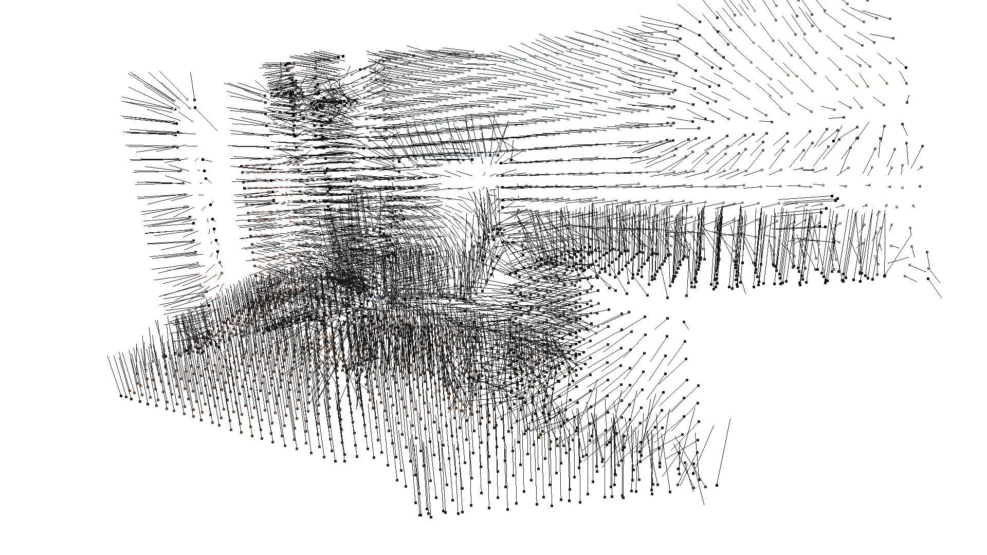
estimate_normals computes the normal for every point. The function finds adjacent points and calculates the principal axis of the adjacent points using covariance analysis.
The function takes an instance of KDTreeSearchParamHybrid class as an argument. The two key arguments radius = 0.1 and max_nn = 30 specifies search radius and maximum nearest neighbor. It has 10cm of search radius, and only considers up to 30 neighbors to save computation time.
Note:
The covariance analysis algorithm produces two opposite directions as normal candidates. Without knowing the global structure of the geometry, both can be correct. This is known as the normal orientation problem. CloudViewer tries to orient the normal to align with the original normal if it exists. Otherwise, CloudViewer does a random guess. Further orientation functions such as orient_normals_to_align_with_direction and orient_normals_towards_camera_location need to be called if the
orientation is a concern.
Access estimated vertex normal#
Estimated normal vectors can be retrieved from the normals variable of downpcd.
[5]:
print("Print a normal vector of the 0th point")
print(downpcd.get_normal(0))
Print a normal vector of the 0th point
[-0.27544311 -0.89184016 -0.3588205 ]
To check out other variables, please use help(downpcd). Normal vectors can be transformed as a numpy array using np.asarray.
[6]:
print("Print the normal vectors of the first 10 points")
print(np.asarray(downpcd.get_normals())[:10, :])
Print the normal vectors of the first 10 points
[[-0.27544311 -0.89184016 -0.3588205 ]
 [-0.04332085 -0.99415791 -0.0988604 ]
 [-0.00301411 -0.99967998 -0.02511759]
 [-0.93796945 -0.07255741  0.33904099]
 [-0.4349595  -0.62494183 -0.64827299]
 [-0.09848166 -0.99274033 -0.06905036]
 [-0.27598658 -0.67162049 -0.68757349]
 [-0.11693341 -0.95517516 -0.27196872]
 [-0.00907847 -0.99964076 -0.02521798]
 [-0.11023104 -0.99207938 -0.06022933]]
Check Working with NumPy for more examples regarding numpy arrays.
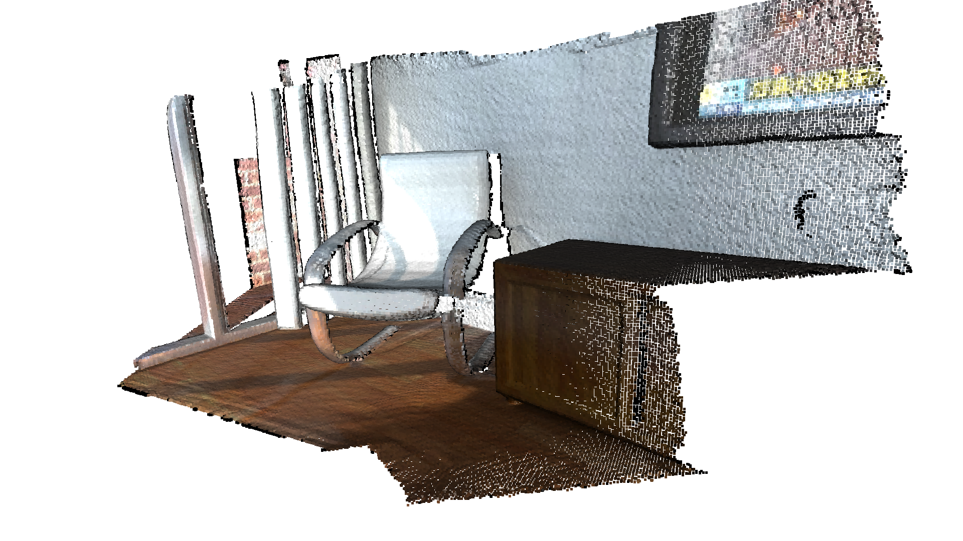
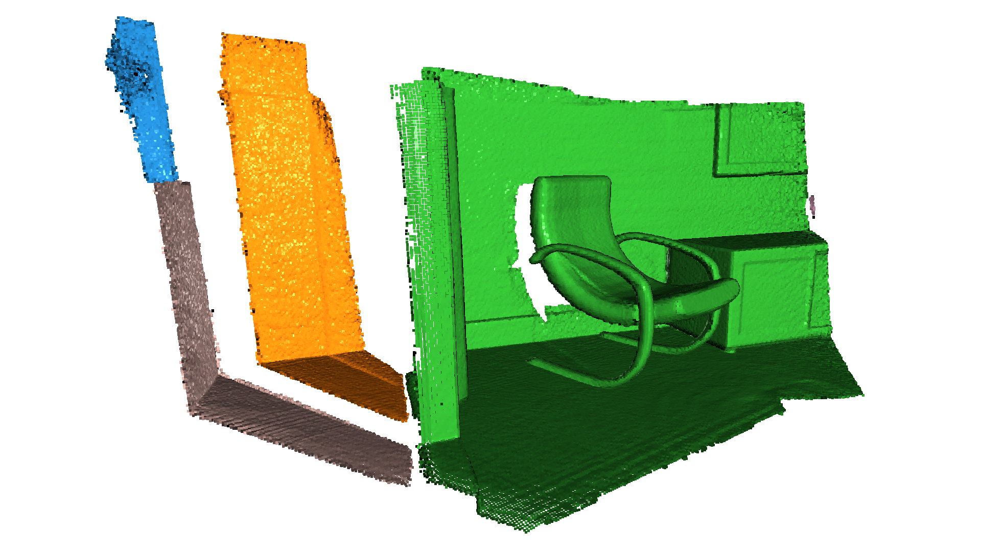
Crop point cloud#
[7]:
print("Load a polygon volume and use it to crop the original point cloud")
demo_crop_data = cv3d.data.DemoCropPointCloud()
pcd = cv3d.io.read_point_cloud(demo_crop_data.point_cloud_path)
vol = cv3d.visualization.read_selection_polygon_volume(
    demo_crop_data.cropped_json_path)
chair = vol.crop_point_cloud(pcd)
cv3d.visualization.draw_geometries([chair],
                                   zoom=0.7,
                                   front=[0.5439, -0.2333, -0.8060],
                                   lookat=[2.4615, 2.1331, 1.338],
                                   up=[-0.1781, -0.9708, 0.1608])
Load a polygon volume and use it to crop the original point cloud
[CloudViewer WARNING] GLFW initialized for headless rendering.

read_selection_polygon_volume reads a json file that specifies polygon selection area. vol.crop_point_cloud(pcd) filters out points. Only the chair remains.
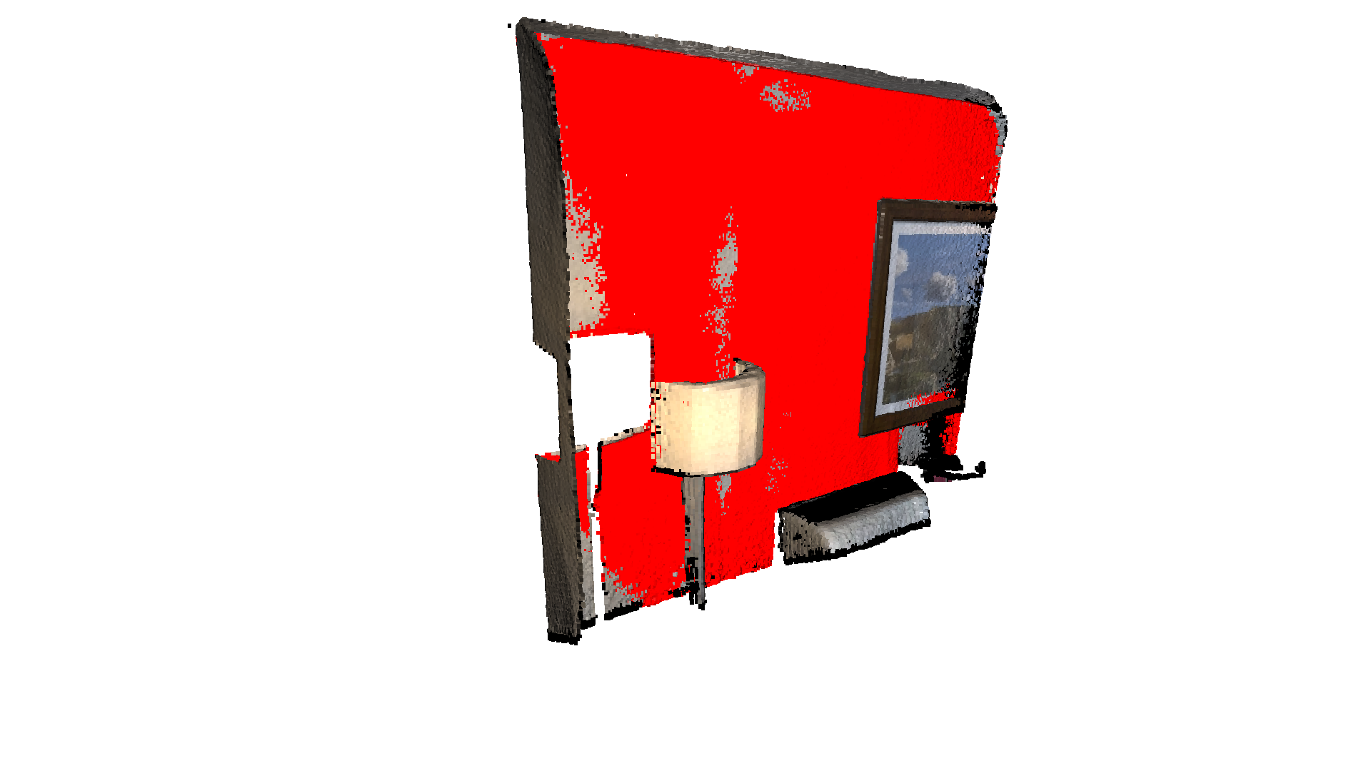
Paint point cloud#
[8]:
print("Paint chair")
chair.paint_uniform_color([1, 0.706, 0])
cv3d.visualization.draw_geometries([chair],
                                   zoom=0.7,
                                   front=[0.5439, -0.2333, -0.8060],
                                   lookat=[2.4615, 2.1331, 1.338],
                                   up=[-0.1781, -0.9708, 0.1608])
Paint chair
[CloudViewer WARNING] GLFW initialized for headless rendering.
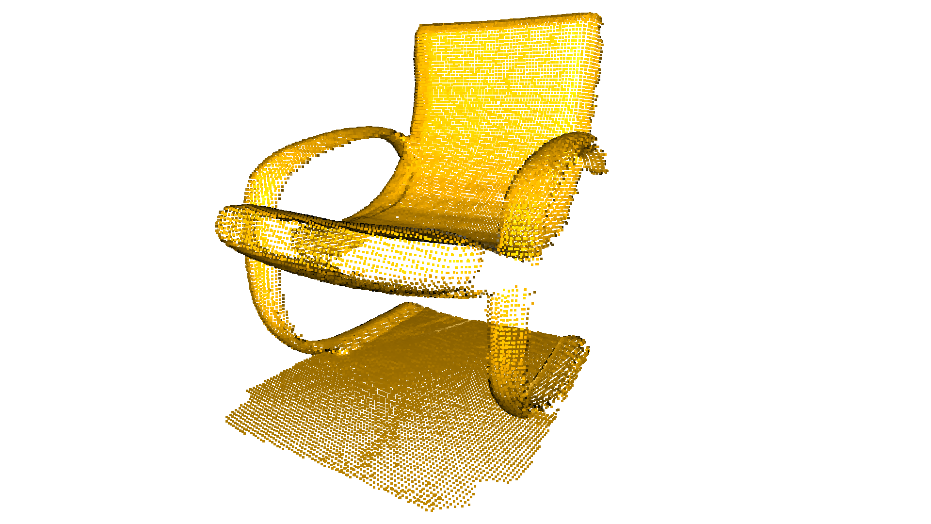
paint_uniform_color paints all the points to a uniform color. The color is in RGB space, [0, 1] range.
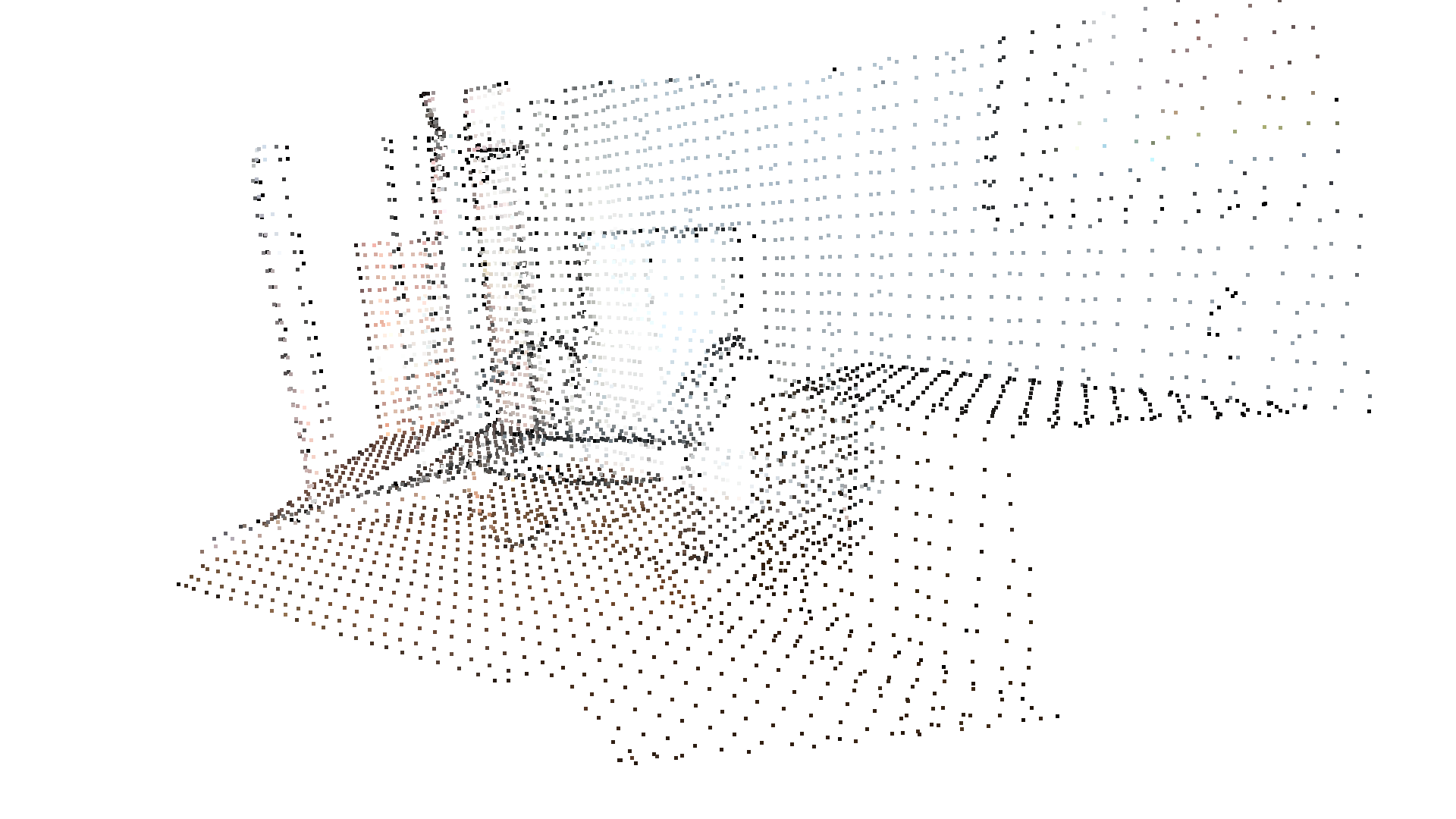
Point cloud distance#
CloudViewer provides the method compute_point_cloud_distance to compute the distance from a source point cloud to a target point cloud. I.e., it computes for each point in the source point cloud the distance to the closest point in the target point cloud.
In the example below we use the function to compute the difference between two point clouds. Note that this method could also be used to compute the Chamfer distance between two point clouds.
[9]:
# Load data
demo_crop_data = cv3d.data.DemoCropPointCloud()
pcd = cv3d.io.read_point_cloud(demo_crop_data.point_cloud_path)
vol = cv3d.visualization.read_selection_polygon_volume(
    demo_crop_data.cropped_json_path)
chair = vol.crop_point_cloud(pcd)

dists = pcd.compute_point_cloud_distance(chair)
dists = np.asarray(dists)
ind = np.where(dists > 0.01)[0]
pcd_without_chair = pcd.select_by_index(ind)
cv3d.visualization.draw_geometries([pcd_without_chair],
                                   zoom=0.3412,
                                   front=[0.4257, -0.2125, -0.8795],
                                   lookat=[2.6172, 2.0475, 1.532],
                                   up=[-0.0694, -0.9768, 0.2024])
[CloudViewer WARNING] GLFW initialized for headless rendering.
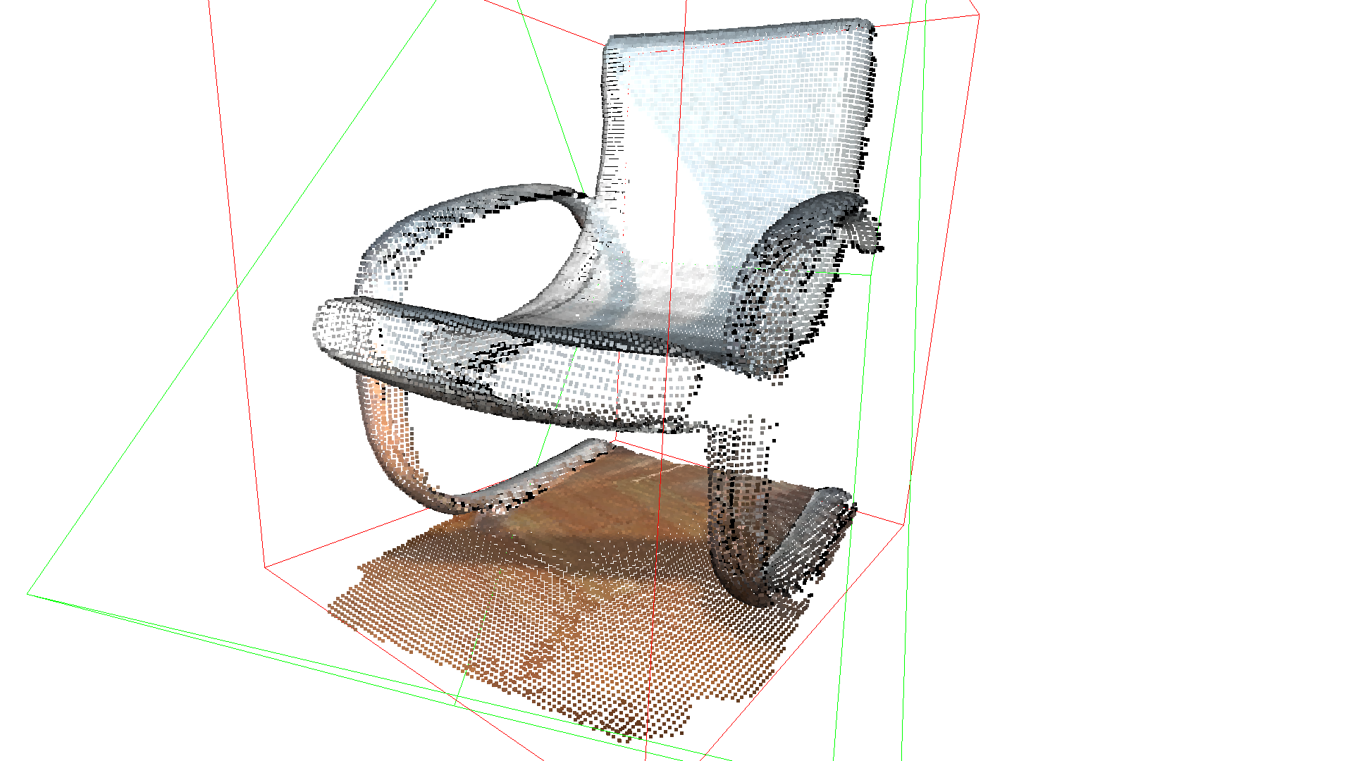
Bounding volumes#
The PointCloud geometry type has bounding volumes as all other geometry types in CloudViewer. Currently, CloudViewer implements an AxisAlignedBoundingBox and an OrientedBoundingBox that can also be used to crop the geometry.
[10]:
aabb = chair.get_axis_aligned_bounding_box()
aabb.set_color((1, 0, 0))
obb = chair.get_oriented_bounding_box()
obb.set_color((0, 1, 0))
cv3d.visualization.draw_geometries([chair, aabb, obb],
                                   zoom=0.7,
                                   front=[0.5439, -0.2333, -0.8060],
                                   lookat=[2.4615, 2.1331, 1.338],
                                   up=[-0.1781, -0.9708, 0.1608])
[CloudViewer WARNING] GLFW initialized for headless rendering.
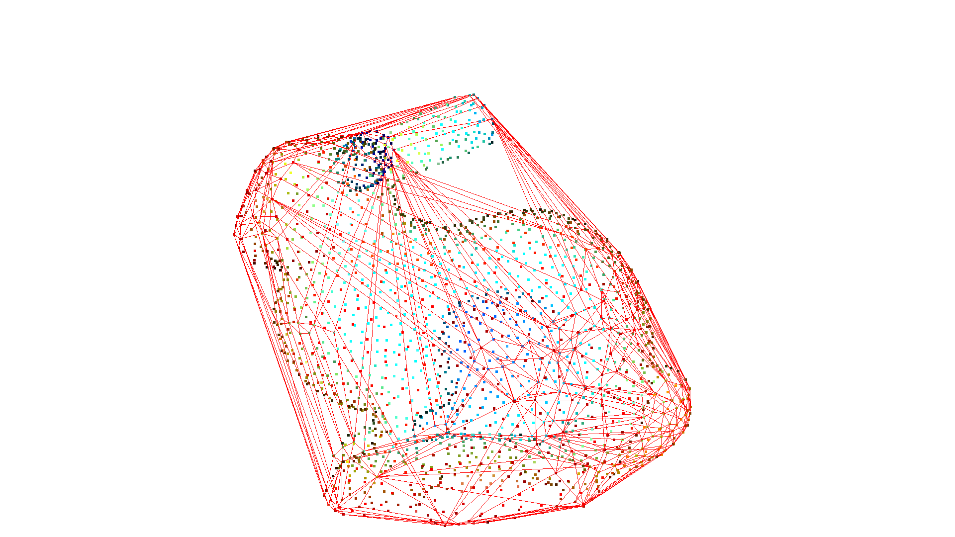
Convex hull#
The convex hull of a point cloud is the smallest convex set that contains all points. CloudViewer contains the method compute_convex_hull that computes the convex hull of a point cloud. The implementation is based on Qhull.
In the example code below we first sample a point cloud from a mesh and compute the convex hull that is returned as a triangle mesh. Then, we visualize the convex hull as a red LineSet.
[11]:
bunny = cv3d.data.BunnyMesh()
mesh = cv3d.io.read_triangle_mesh(bunny.path)
mesh.compute_vertex_normals()
pcl = mesh.sample_points_poisson_disk(number_of_points=2000)
hull, _ = pcl.compute_convex_hull()
hull_ls = cv3d.geometry.LineSet.create_from_triangle_mesh(hull)
hull_ls.paint_uniform_color((1, 0, 0))
cv3d.visualization.draw_geometries([pcl, hull_ls])
[CloudViewer WARNING] GLFW initialized for headless rendering.
DBSCAN clustering#
Given a point cloud from e.g. a depth sensor we want to group local point cloud clusters together. For this purpose, we can use clustering algorithms. CloudViewer implements DBSCAN [Ester1996] that is a density based clustering algorithm. The algorithm is implemented in cluster_dbscan and requires two parameters: eps defines the distance to neighbors in a cluster and min_points defines the minimum number of points required to form a cluster. The
function returns labels, where the label -1 indicates noise.
[12]:
ply_point_cloud = cv3d.data.PLYPointCloud()
pcd = cv3d.io.read_point_cloud(ply_point_cloud.path)

with cv3d.utility.VerbosityContextManager(
        cv3d.utility.VerbosityLevel.Debug) as cm:
    labels = np.array(
        pcd.cluster_dbscan(eps=0.02, min_points=10, print_progress=True))

max_label = labels.max()
print(f"point cloud has {max_label + 1} clusters")
colors = plt.get_cmap("tab20")(labels / (max_label if max_label > 0 else 1))
colors[labels < 0] = 0
pcd.set_colors(cv3d.utility.Vector3dVector(colors[:, :3]))
cv3d.visualization.draw_geometries([pcd],
                                   zoom=0.455,
                                   front=[-0.4999, -0.1659, -0.8499],
                                   lookat=[2.1813, 2.0619, 2.0999],
                                   up=[0.1204, -0.9852, 0.1215])
[CloudViewer DEBUG] Precompute Neighbours
[CloudViewer DEBUG] Done Precompute Neighbours
[CloudViewer DEBUG] Compute Clusters
[CloudViewer DEBUG] Done Compute Clusters: 10
Precompute Neighbours[========================================] 100%
point cloud has 10 clusters
[CloudViewer WARNING] GLFW initialized for headless rendering.
Note:
This algorithm precomputes all neighbors in the epsilon radius for all points. This can require a lot of memory if the chosen epsilon is too large.
Plane segmentation#
CloudViewer also supports segmententation of geometric primitives from point clouds using RANSAC. To find the plane with the largest support in the point cloud, we can use segment_plane. The method has three arguments: distance_threshold defines the maximum distance a point can have to an estimated plane to be considered an inlier, ransac_n defines the number of points that are randomly sampled to estimate a plane, and num_iterations defines how often a random plane is sampled
and verified. The function then returns the plane as \((a,b,c,d)\) such that for each point \((x,y,z)\) on the plane we have \(ax + by + cz + d = 0\). The function further returns a list of indices of the inlier points.
[13]:
pcd_point_cloud = cv3d.data.PCDPointCloud()
pcd = cv3d.io.read_point_cloud(pcd_point_cloud.path)
plane_model, inliers = pcd.segment_plane(distance_threshold=0.01,
                                         ransac_n=3,
                                         num_iterations=1000)
[a, b, c, d] = plane_model
print(f"Plane equation: {a:.2f}x + {b:.2f}y + {c:.2f}z + {d:.2f} = 0")

inlier_cloud = pcd.select_by_index(inliers)
inlier_cloud.paint_uniform_color([1.0, 0, 0])
outlier_cloud = pcd.select_by_index(inliers, invert=True)
cv3d.visualization.draw_geometries([inlier_cloud, outlier_cloud],
                                   zoom=0.8,
                                   front=[-0.4999, -0.1659, -0.8499],
                                   lookat=[2.1813, 2.0619, 2.0999],
                                   up=[0.1204, -0.9852, 0.1215])
Plane equation: -0.06x + -0.10y + 0.99z + -1.06 = 0
[CloudViewer WARNING] GLFW initialized for headless rendering.
Hidden point removal#
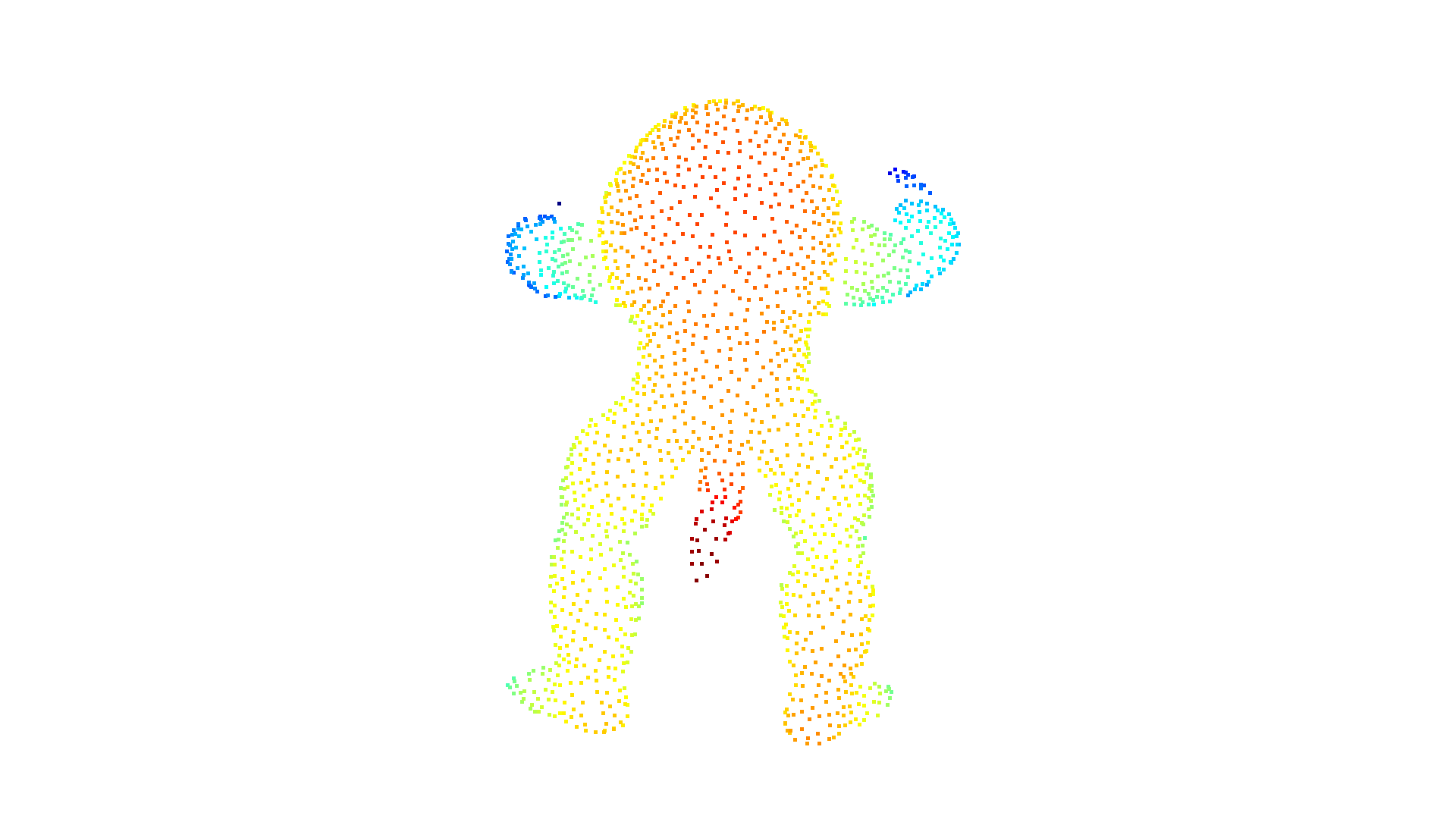
Imagine you want to render a point cloud from a given view point, but points from the background leak into the foreground because they are not occluded by other points. For this purpose we can apply a hidden point removal algorithm. In CloudViewer the method by [Katz2007] is implemented that approximates the visibility of a point cloud from a given view without surface reconstruction or normal estimation.
[14]:
print("Convert mesh to a point cloud and estimate dimensions")
armadillo_data = cv3d.data.ArmadilloMesh()
pcd = cv3d.io.read_triangle_mesh(
    armadillo_data.path).sample_points_poisson_disk(5000)
diameter = np.linalg.norm(
    np.asarray(pcd.get_max_bound()) - np.asarray(pcd.get_min_bound()))
cv3d.visualization.draw_geometries([pcd])
Convert mesh to a point cloud and estimate dimensions
[CloudViewer WARNING] GLFW initialized for headless rendering.
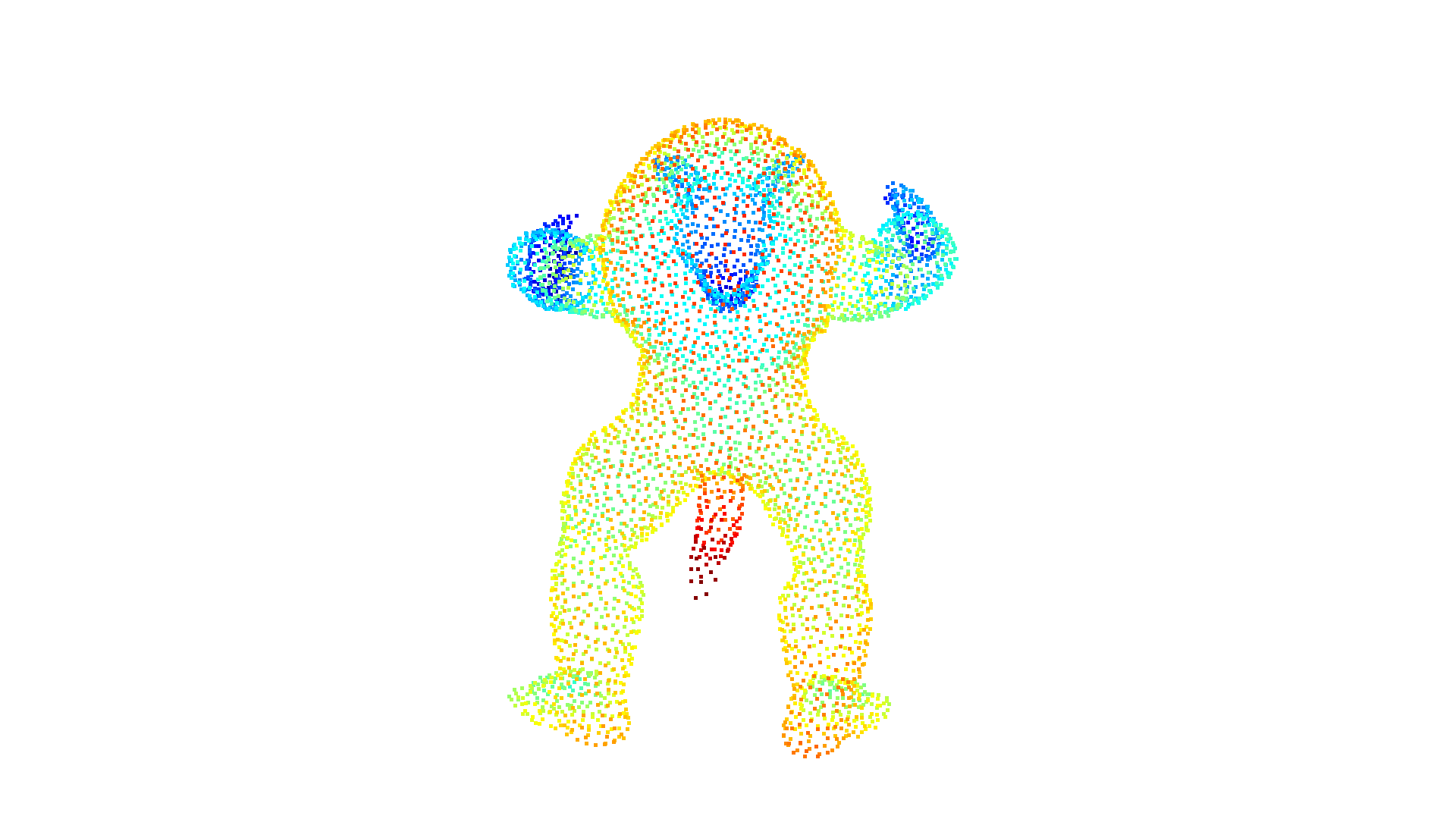
[15]:
print("Define parameters used for hidden_point_removal")
camera = [0, 0, diameter]
radius = diameter * 100

print("Get all points that are visible from given view point")
_, pt_map = pcd.hidden_point_removal(camera, radius)

print("Visualize result")
pcd = pcd.select_by_index(pt_map)
cv3d.visualization.draw_geometries([pcd])
Define parameters used for hidden_point_removal
Get all points that are visible from given view point
Visualize result
[CloudViewer WARNING] GLFW initialized for headless rendering.